In this article, we set out how the OBR's economic and fiscal forecasts capture the dynamic effects of policies on the economic behaviour of people and businesses.

Dynamic scoring (or dynamic costing) is a method of estimating the total fiscal impact of a given policy change which takes account of its secondary (or ‘indirect’) impact on the economy as a result of the dynamic response of people and businesses that are affected. Dynamic scoring can be distinguished from static scoring (or static costing) which only considers the direct (or first round) impact of a given policy change on the public finances. Taking the example of a 1 percentage point reduction in the rate of corporation tax:

• a static scoring would apply the difference in tax rates to the same level of corporate profits to estimate the associated reduction in tax revenues over the forecast period. This estimate of the ‘direct’ cost of the policy assumes there is no change in the behaviour of corporations or any other actor in the economy in response to the tax cut.

• a dynamic scoring would start from the same estimate of the direct fiscal cost but also take account of the increase in corporate investment that could arise from the resulting increase in post-tax corporate profits. By raising the economy-wide capital stock, productivity, and output, and thereby boosting household earnings and consumption, this increase in investment could also increase the yield from other taxes like income tax and VAT. These ‘second round’ or ‘indirect’ effects of the policy measure can thereby offset some of its static or ‘direct’ fiscal cost over the forecast period.

The OBR never presents purely static estimates of the fiscal impact of individual policy measures, except where it has considered dynamic effects and deemed them to be so small as to be negligible. In estimating the overall fiscal impact of policy measures, the OBR takes three kinds of dynamic effects into account:

Within the costings of individual policy measures, we incorporate any behavioural effects which we think are likely to be large enough to materially effect their direct cost or yield. For example, when estimating the revenue impact of a reduction in the rate of fuel duty, we take account of what our models predict will be the increase in fuel consumption in response to the lower cost of motoring. This slightly offsets the ‘static’ revenue loss from simply reducing the per litre rate of duty. Other behavioural responses can include, for example, how taxpayers respond to new tax incentives – both by increasing the activity that policymakers wish to incentivise but also by activities designed to minimise their overall tax liability. You can read more about how we cost individual policies in Briefing paper No. 6: Policy costings and our forecast.

In our forecast of aggregate demand, we also estimate the economic impact of the whole package of policies in a given Budget or fiscal statement using our published fiscal multipliers. These fiscal multipliers vary by class of policy instrument and estimate the impact of each on aggregate demand, based on past historical relationships. For example, public investment changes have a first-year multiplier of 1 (i.e. £1 of additional public investment generates £1 of additional real GDP in the first year) while income tax changes have a multiplier of 0.3 in the year they are announced.

Multipliers differ due to the extent to which beneficiaries might save rather than spend additional funds, or the extent to which spending goes on imports rather than domestic output. All of these multipliers are assumed to taper to zero over five years, as the initial boost to aggregate demand is eventually offset by changes in monetary policy, the exchange rate, and real wages which bring output back into line with its long-run potential. In this way, the temporary demand effects of all policies are taken into account in our economy forecast and fed back into our fiscal forecasts. For example, where governments loosen fiscal policy (i.e. increase borrowing), they tend to recoup part of that additional borrowing via the revenues generated by the short-term stimulus to incomes and consumption. The demand multipliers that we currently use in our fiscal forecasts are shown in the table below. These multipliers are kept under regular review and adapted to the policies in question and changing macroeconomic environment, as highlighted in Box 2.2 of our December 2019 Forecast evaluation report and Box 2.1 of our November 2020 Economic and fiscal outlook (EFO).

OBR fiscal multipliers

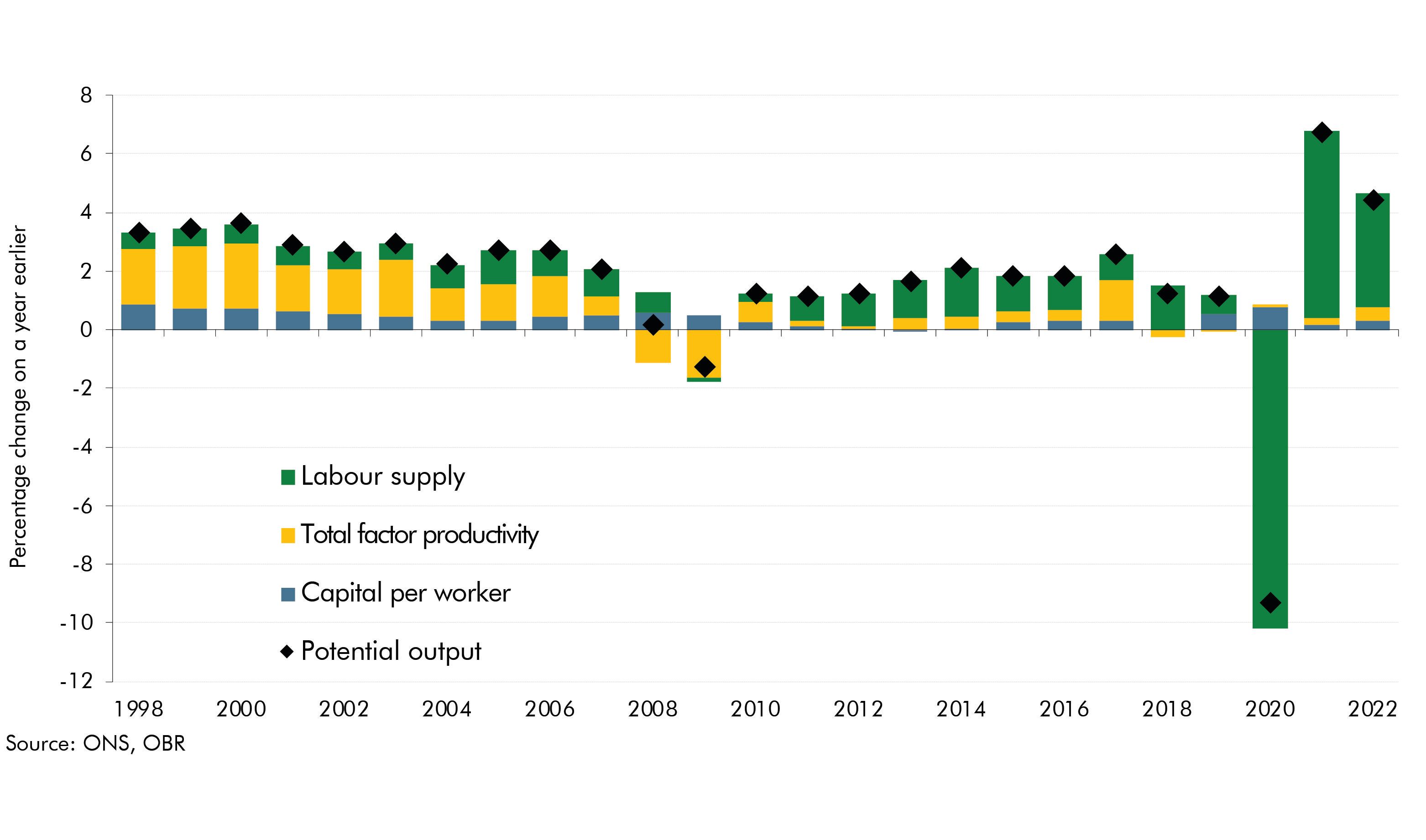
In our forecast of the supply side of the economy, we also take account of specific policies which evidence suggests are likely to have a significant, additional, and durable effect on the potential output of the economy. Based on standard growth accounting models, we capture the supply side effects of policies via their impact on three key determinants of the productive potential of the economy. These are (i) the labour supply, (ii) the capital stock, and (iii) ‘total factor productivity’ (the efficiency with which labour and capital are combined to produce goods and services). The contribution that each of the supply determinants has made to overall GDP growth over the past 25 years is shown in the chart below. Unlike demand effects, supply side effects are estimated on a policy-by-policy basis and can be permanent if they deliver a lasting change in the level of employment, level of investment, or economy-wide level of productivity. You can read more about how we account for the supply side effects of policies in our forecasts in Briefing paper No. 8: Forecasting potential output – the supply side of the economy.

Supply-side drivers of potential output growth, 1998-2022

Most of our costings of tax and welfare policy changes incorporate behavioural changes, some of which can significantly impact the overall yield or cost of the policy. For example:

• Increases in tobacco duty raise far less revenue than one might expect from the static costing. As we explained in our October 2021 EFO, the dynamic effect of an increase in duty is so large that around 80 per cent of the static yield is assumed to be lost to the behavioural response. Indeed, the evidence suggests that the duty rate for cigarettes is beyond the peak of the ‘Laffer curve’, the revenue maximising rate of tax. We capture this type of behavioural response through the use of price elasticities of demand, which estimate the impact of higher duty on cigarette consumption but also the demand for related products, such as hand-rolled tobacco, as well as the incentive to switch to alternative suppliers, such as those in the illicit market.
• Changes in the rates of personal taxation for high-income individuals have repeatedly led to large behavioural responses. For example, the March 2012 Budget decision to cut the top rate of income tax from 50 to 45p had a ‘static costing’ (ignoring behavioural effects) of £3.8 billion in lower revenue by 2015-16. However, once likely behavioural response on the part of taxpayers was taken into account (in the form of both changes in hours worked and ‘tax planning’) the OBR’s central estimate of the loss of revenue was reduced to just £100 million. HMRC’s published analysis suggested the old and new rates straddled the revenue maximising rate of 48p.
• Behavioural responses to changes in welfare benefits generally fall into one of three categories: the proportion of those eligible for a benefit that actually claim it, the degree to which a change in policy for one benefit can have knock-on implications to the spending of a related benefit, and thirdly, whether a claimant seeks to or is able to change their circumstances in response to a policy change. The 2013 introduction of the benefit cap, which capped the housing benefit award for certain households, is a good example of a costing where we had to consider several potential behavioural responses. Those affected by the cap might seek to switch to exempt benefits, they may decide to move into work, they may decide to move to lower-rent homes, and some couples might choose to separate so that a lower cap would apply. Our current view is that the observed behavioural responses lowered the costing of the measure by around half.¹
  

Our economic and fiscal forecasts have also systematically incorporated the net effects of the Government’s policies on aggregate demand. In the 26 forecasts we have produced in the 13 years in which the OBR has been in operation, fiscal policy has delivered a net stimulus to demand in 12, a net reduction in demand in 8, and been broadly demand neutral in 6 of those forecasts. For example, our most recent March 2023 forecast assumed that the package of spending increases, and tax reductions announced in the 2023 Spring Budget would increase the level of real GDP by around 0.3 per cent in 2023-24 and 2024-25, with the effect tapering to zero by 2027-28.

Finally, our economic and fiscal forecasts have taken account of the impacts of policies on the supply side of the economy, where those effects are expected to be material, additional, and durable. For example:

• In July 2015 the government announced the introduction of the National Living Wage from April 2016. We assumed that the increase in firms’ wage costs would increase the level of structural unemployment by 60,000 in 2020 and reduce overall labour supply (employment and hours) by 0.4 per cent. This was equivalent to a reduction in potential output of 0.1 per cent by 2020.
• In March 2020 the Government announced plans to increase public sector capital spending permanently by more than 30 per cent in real terms. We estimated that, if this were to transpire, it would gradually but significantly increase the public sector capital stock – by around a quarter over the long term. The full effects would be felt well beyond our five-year forecast horizon but could have led to an eventual increase in the size of the economy of around 2.5 per cent.
• Most recently, in our March 2023 forecast we incorporated our expectation that the Chancellor’s childcare and other labour market policies would increase employment by 110,000 and potential output by 0.2 per cent in five years.

As these examples demonstrate, OBR forecasts systematically incorporate the dynamic effects of policies on the economic behaviour– be it personal retirement decisions, company investment decisions, or decisions by those not currently in the labour force to seek work – drawing on a wide range of empirical estimates. We sought feedback on our approach over the summer of 2023 and are open to any evidence on how these approaches could be improved, including on whether the dynamic effects reflected in our forecasts may be too large or too small.

Acknowledgements

We are grateful for the engagement, expertise, and insights from various OBR staff members in compiling this article.

Downloads

Dynamic scoring of policy measures in OBR forecasts (article PDF)